Concept 9: Introduction to Generative Models
Introduction to Generative Models
ℹ️ Definition Generative Models are machine learning models that learn the underlying probability distribution of data to generate new, realistic samples that resemble the training data, enabling applications like image synthesis, text generation, and content creation.
Learning Objectives
By the end of this lesson, you will:
- Understand the difference between generative and discriminative models
- Learn the core concepts of probability distributions and sampling
- Explore types of generative models (explicit vs implicit density)
- Understand latent space representations
- Implement a simple Gaussian Mixture Model (GMM)
- Preview VAEs, GANs, Diffusion Models, and Transformers
Introduction
In Lessons 1-8, we learned Reinforcement Learning - teaching agents to make decisions through trial and error. Now we shift to a different paradigm: Generative AI - teaching models to create new content.
Examples of Generative AI:
- DALL-E 3: Text -> Image generation
- GPT-4: Text completion and generation
- Stable Diffusion: Image synthesis from text
- Midjourney: Artistic image creation
- GitHub Copilot: Code generation
These systems generate new content that resembles their training data but is novel.
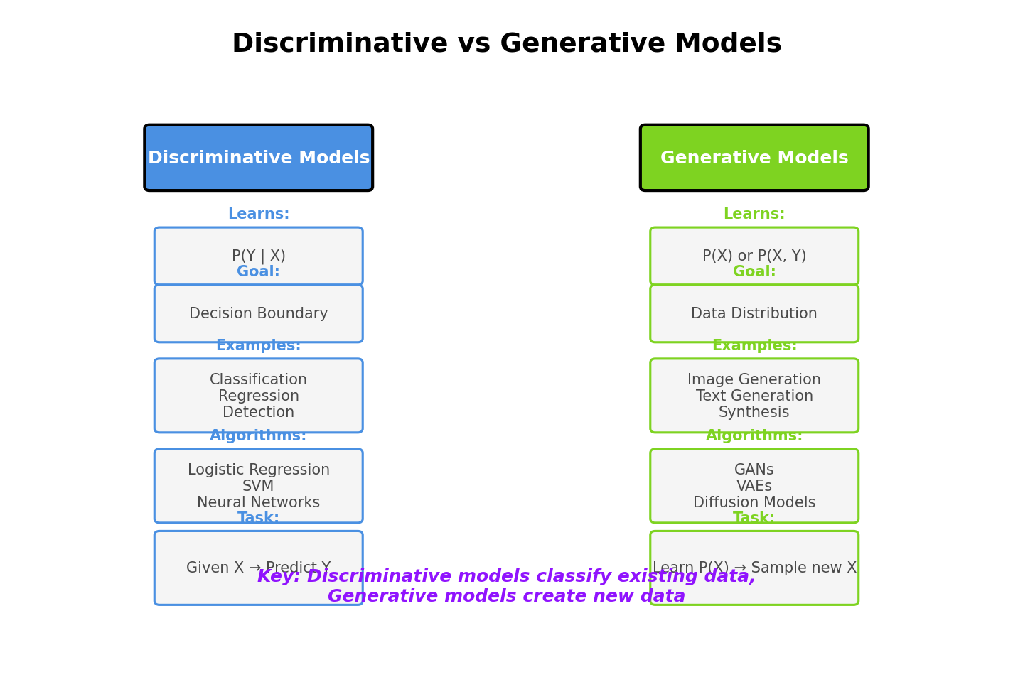
Discriminative vs Generative Models
Discriminative Models
Goal: Learn the boundary between classes
Examples:
- Image classification: "Is this a cat or dog?"
- Spam detection: "Is this email spam or not?"
- Object detection: "Where are the cars in this image?"
Model: P(y|x) - Probability of label y given input x
Analogy: A discriminative model is like a judge who can tell real paintings from fakes, but can't create paintings.
Generative Models
Goal: Learn the distribution of data to generate new samples
Examples:
- Image generation: "Create a realistic face"
- Text generation: "Complete this sentence"
- Music generation: "Compose a symphony"
Model: P(x) - Probability distribution of data x
Analogy: A generative model is like an artist who can create new paintings that look real.
Comparison
| Aspect | Discriminative | Generative |
|---|---|---|
| Learns | Decision boundary | Data distribution |
| Model | P(y|x) | P(x) or P(x,y) |
| Task | Classification, regression | Generation, sampling |
| Example | "Is this a dog?" | "Generate a dog image" |
| Difficulty | Easier (lower-dimensional) | Harder (high-dimensional) |
Can do both:
- Generative models can classify: P(y|x) = P(x|y) * P(y) / P(x) (Bayes' rule)
- But discriminative models cannot generate
Core Concepts
Probability Distributions
Generative models learn: P(x) = probability distribution over data
Example - 1D Data (Heights):
css
Heights ~ N(μ=170cm, σ=10cm)

P(height=180cm) = [probability density]

To generate new samples: sample from N(170, 10)
Example - High-Dimensional (Images):
python
Images: 256×256 RGB = 196,608 dimensions
P(x) over all possible images is intractably complex!

Generative models approximate P(x) with neural networks
Sampling
Sampling: Drawing new data points from learned distribution
python
# Simple example: Gaussian distribution
mu, sigma = 0, 1
sample = np.random.normal(mu, sigma)  # Generate new data point

# Generative model: Complex distribution
latent_code = np.random.randn(128)  # Random noise
generated_image = generator(latent_code)  # Generate image
Likelihood
Likelihood: How probable is observed data under our model?
css
Likelihood = P(x | model parameters)

High likelihood: Model explains data well
Low likelihood: Model doesn't fit data
Training objective: Maximize likelihood of training data
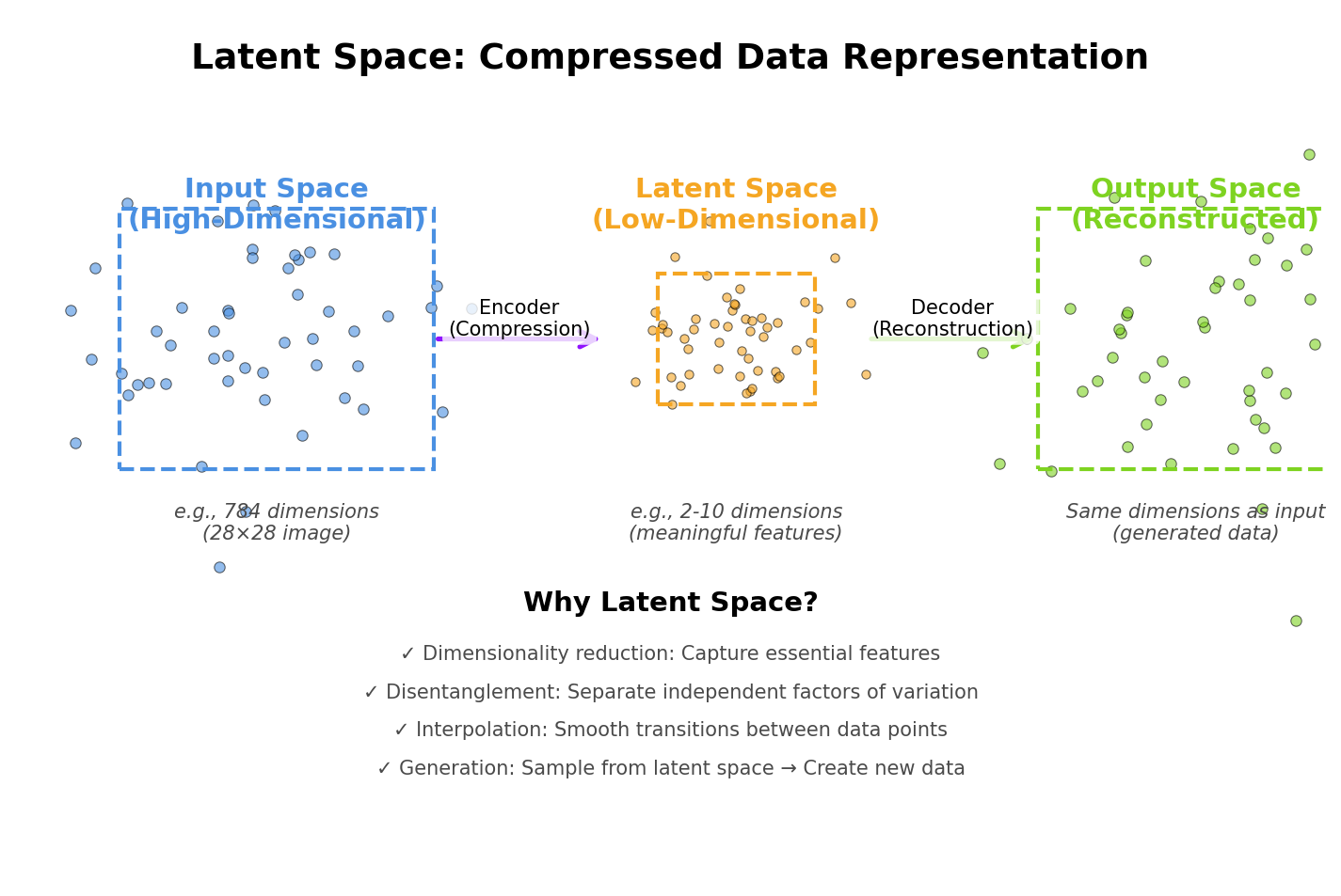
Latent Space
Latent space: Low-dimensional representation of high-dimensional data
Intuition:
- Data space: Images (256x256x3 = 196K dimensions)
- Latent space: Codes (128 dimensions)
- Key idea: Meaningful structure in latent space
Example:
css
Latent code [0.5, 0.2, -0.3, ...] → Image of "young man with beard"
Latent code [0.6, 0.3, -0.2, ...] → Image of "young woman with smile"
                ↑
         Smooth interpolation possible!
Operations in latent space:
ini
man_with_glasses = man + glasses - face
woman_with_glasses = woman + glasses - face

This arithmetic works because latent space has structure!
Types of Generative Models
Explicit Density Models
Explicitly model P(x)
Advantages:
- Can compute exact likelihood
- Principled training objective
- Interpretable
Disadvantages:
- Often restrictive assumptions
- Can be slow to sample from
Examples:
-
Autoregressive Models (PixelCNN, GPT)
- Decompose P(x) = P(x₁) * P(x₂|x₁) * P(x₃|x₁,x₂) * ...
- Generate pixel-by-pixel or token-by-token
-
Variational Autoencoders (VAEs)
- Approximate P(x) using latent variables
- Optimize Evidence Lower Bound (ELBO)
-
Normalizing Flows
- Transform simple distribution to complex one
- Exact likelihood computation
Implicit Density Models
Don't explicitly model P(x), just generate samples
Advantages:
- More flexible (no distributional assumptions)
- Often generate higher-quality samples
- Faster sampling
Disadvantages:
- No likelihood computation
- Training can be unstable
- Harder to evaluate
Examples:
-
Generative Adversarial Networks (GANs)
- Generator creates samples
- Discriminator judges real vs fake
- Adversarial training
-
Diffusion Models
- Gradually denoise random noise
- Implicit but tractable generation process

Common Generative Model Architectures
One. Gaussian Mixture Models (GMM)
Simple generative model: Data comes from mixture of Gaussians
css
P(x) = Σ_k π_k * N(x | μ_k, Σ_k)
Where:
- K: Number of components
- π_k: Mixture weight for component k
- μ_k, Σ_k: Mean and covariance of component k
Generation:
- Sample component k ~ Categorical(π)
- Sample x ~ N(μ_k, Σ_k)
Training: Expectation-Maximization (EM) algorithm
2. Variational Autoencoders (VAEs)
Architecture:
vbnet
Encoder: x → z (infer latent code from data)
Decoder: z → x̂ (reconstruct data from latent code)
Training objective:
perl
ELBO = E_q[log p(x|z)] - KL(q(z|x) || p(z))
        ↑                  ↑
   Reconstruction     Regularization
Generation:
- Sample z ~ N(0, I)
- Generate x = decoder(z)
3. Generative Adversarial Networks (GANs)
Architecture:
makefile
Generator: z → x (create fake samples)
Discriminator: x → [0,1] (judge real vs fake)
Training: Adversarial game
css
Generator: Fool discriminator (generate realistic samples)
Discriminator: Distinguish real from fake

min_G max_D E[log D(x)] + E[log(1 - D(G(z)))]
4. Diffusion Models
Idea: Gradually add noise to data, then learn to reverse the process
Forward process (diffusion):
scss
x₀ → x₁ → x₂ → ... → x_T ~ N(0,I)
Reverse process (generation):
scss
x_T ~ N(0,I) → x_{T-1} → ... → x₁ → x₀
Generation: Start from noise, iteratively denoise
5. Autoregressive Models (Transformers)
Idea: Model P(x) as product of conditional probabilities
css
P(x₁, x₂, ..., x_n) = P(x₁) * P(x₂|x₁) * P(x₃|x₁,x₂) * ...
Generation: Sequential sampling
css
Sample x₁ ~ P(x₁)
Sample x₂ ~ P(x₂|x₁)
Sample x₃ ~ P(x₃|x₁,x₂)
...
Examples: GPT (text), PixelCNN (images)
Evaluation Metrics
For Image Generation
One. Inception Score (IS)
- Measures quality and diversity
- Higher is better
- Range: 1 (worst) to ∞
2. Fréchet Inception Distance (FID)
- Measures similarity to real data distribution
- Lower is better
- Range: 0 (perfect) to ∞
3. Human Evaluation
- Show generated samples to humans
- Ask: "Is this real or generated?"
- "Which image looks better?"
For Text Generation
One. Perplexity
- Measures how well model predicts text
- Lower is better
2. BLEU/ROUGE/METEOR
- Compare generated text to reference
- Measures n-gram overlap
3. Human Evaluation
- Fluency, coherence, factuality
- Turing test: Can humans distinguish?
General Metrics
One. Likelihood (if computable)
- P(x) for test data
- Higher is better
2. Sample Quality
- Visual inspection
- Diversity of generations
- Mode coverage
3. Interpolation
- Smooth transitions in latent space?
- Meaningful arithmetic?
Applications of Generative Models
Computer Vision
Image Synthesis:
- DALL-E 3, Midjourney, Stable Diffusion
- Text-to-image generation
- Style transfer
Image-to-Image Translation:
- Day -> Night, Summer -> Winter
- Sketch -> Photo
- Low-resolution -> High-resolution (super-resolution)
Image Editing:
- Inpainting (fill missing regions)
- Outpainting (extend beyond boundaries)
- Object removal/addition
Natural Language Processing
Text Generation:
- GPT-4, Claude, Gemini
- Story writing, code generation, dialogue
Translation:
- Machine translation (English -> French)
- Style transfer (formal -> casual)
Summarization:
- Generate concise summaries from long documents
Audio and Music
Speech Synthesis:
- Text-to-speech (TTS)
- Voice cloning
- Accent conversion
Music Generation:
- Compose melodies
- Generate backing tracks
- Style transfer (classical -> jazz)
Scientific Applications
Drug Discovery:
- Generate novel molecular structures
- Optimize drug properties
Protein Design:
- Generate functional proteins
- AlphaFold for structure prediction
Materials Science:
- Design new materials with desired properties
Challenges in Generative Modeling
One. Mode Collapse
Problem: Model generates limited variety of samples
Example:
- GAN trained on faces only generates a few distinct faces
- Missing diversity in training data
Solutions:
- Minibatch discrimination
- Feature matching
- Multiple discriminators
2. Training Instability
Problem: Training diverges or oscillates
Example:
- GAN discriminator becomes too strong
- Generator loss explodes or vanishes
Solutions:
- Careful learning rate tuning
- Gradient penalty (WGAN-GP)
- Progressive training
3. Evaluation Difficulty
Problem: Hard to measure generation quality
Challenge:
- No single perfect metric
- Human evaluation expensive
- Likelihood doesn't correlate with quality
Solutions:
- Use multiple metrics (FID, IS, perplexity)
- Downstream task performance
- Human evaluation studies
4. Computational Cost
Problem: Training generative models is expensive
Example:
- Stable Diffusion: trained on 600M images
- GPT-3: 300B tokens, $4.6M training cost
- DALL-E 3: Billions of image-text pairs
Solutions:
- Smaller models for specific domains
- Transfer learning and fine-tuning
- Distillation from large models
Generative AI Ethics
Concerns
One. Deepfakes
- Realistic fake videos/images
- Misinformation and fraud
- Identity theft
2. Copyright and Ownership
- Models trained on copyrighted data
- Who owns generated content?
- Artist attribution
3. Bias and Fairness
- Models amplify training data biases
- Stereotypes in generated content
- Representational harms
4. Environmental Impact
- Massive computational resources
- Carbon footprint of training large models
Responsible AI Practices
One. Watermarking
- Embed invisible markers in generated content
- Enable detection of AI-generated media
2. Attribution
- Credit data sources and artists
- Transparent about AI involvement
3. Bias Mitigation
- Diverse training data
- Fairness metrics and auditing
- User controls for generation
4. Regulation
- Disclosure requirements
- Consent for training data
- Safety guidelines
Simple Implementation: Gaussian Mixture Model
python
import numpy as np
from scipy.stats import multivariate_normal

class GMM:
    def __init__(self, n_components=3):
        self.n_components = n_components

    def fit(self, X, n_iterations=100):
        n_samples, n_features = X.shape

        # Initialize parameters randomly
        self.weights = np.ones(self.n_components) / self.n_components
        self.means = X[np.random.choice(n_samples, self.n_components, replace=False)]
        self.covariances = [np.eye(n_features) for _ in range(self.n_components)]

        # EM algorithm
        for iteration in range(n_iterations):
            # E-step: Compute responsibilities
            responsibilities = self._e_step(X)

            # M-step: Update parameters
            self._m_step(X, responsibilities)

    def _e_step(self, X):
        # Compute probability of each point under each component
        responsibilities = np.zeros((X.shape[0], self.n_components))
        for k in range(self.n_components):
            responsibilities[:, k] = self.weights[k] * \
                multivariate_normal.pdf(X, self.means[k], self.covariances[k])

        # Normalize
        responsibilities /= responsibilities.sum(axis=1, keepdims=True)
        return responsibilities

    def _m_step(self, X, responsibilities):
        # Update weights, means, covariances
        N_k = responsibilities.sum(axis=0)

        self.weights = N_k / X.shape[0]
        self.means = (responsibilities.T @ X) / N_k[:, np.newaxis]

        for k in range(self.n_components):
            diff = X - self.means[k]
            self.covariances[k] = (responsibilities[:, k, np.newaxis] * diff).T @ diff / N_k[k]

    def sample(self, n_samples=1):
        # Generate new samples
        samples = []
        for _ in range(n_samples):
            # Choose component
            k = np.random.choice(self.n_components, p=self.weights)

            # Sample from component
            sample = np.random.multivariate_normal(self.means[k], self.covariances[k])
            samples.append(sample)

        return np.array(samples)

# Example usage
X = np.random.randn(1000, 2)  # Training data
gmm = GMM(n_components=3)
gmm.fit(X)

# Generate new samples
generated_samples = gmm.sample(n_samples=100)
Key Takeaways
- Generative models learn data distributions to create new samples
- Discriminative vs Generative: Classification vs Generation
- Explicit density (VAEs, autoregressive) vs Implicit density (GANs, diffusion)
- Latent space provides low-dimensional representations
- Evaluation is challenging (FID, IS, perplexity, human judgment)
- Applications span vision, language, audio, science
- Ethics requires careful consideration (deepfakes, bias, copyright)
Looking Ahead
In the next lessons, we'll dive deep into specific generative models:
- Lesson 10: Variational Autoencoders (VAEs)
- Lesson 11: Generative Adversarial Networks (GANs)
- Lesson 12: Advanced GAN Architectures
- Lesson 13: Diffusion Models
- Lesson 14: Transformer Architectures for Generation
- Lesson 15: Large Language Models (LLMs)
Get ready to build state-of-the-art generative AI systems!
Summary
- Generative models learn P(x) to generate new data samples
- Key concepts: Probability distributions, sampling, latent spaces
- Types: Explicit density (VAEs, autoregressive) vs Implicit (GANs, diffusion)
- Architectures: GMM, VAE, GAN, Diffusion, Transformers
- Evaluation: FID, IS, perplexity, human judgment
- Applications: Image synthesis, text generation, audio, drug discovery
- Challenges: Mode collapse, instability, evaluation difficulty, cost
- Ethics: Deepfakes, copyright, bias, environmental impact