Concept 3: Deep Q-Networks (DQN)
Deep Q-Networks (DQN)
ℹ️ Definition Deep Q-Networks (DQN) extend Q-Learning to high-dimensional state spaces by using neural networks as function approximators, enabling RL agents to learn directly from raw sensory input like images.
Learning Objectives
By the end of this lesson, you will:
- Understand why neural networks are needed for complex state spaces
- Learn the DQN architecture and key innovations (experience replay, target networks)
- Implement a DQN agent for CartPole using PyTorch
- Understand the challenges of combining deep learning with Q-Learning
- Visualize training dynamics and diagnose common failure modes
- Apply DQN to Atari games with pixel inputs
Introduction
In Lesson 2, we implemented tabular Q-Learning for FrozenLake, where the Q-table had 16 states x 4 actions = 64 entries. But what if your environment has millions of states?
Example - Atari Pong:
- State: 210x160 RGB image = 100,800 pixels
- Possible states: 256^100,800 ~= 10^240,000 (more than atoms in universe!)
- Q-table size: Impossible to store or learn
Deep Q-Networks solve this by using neural networks to approximate Q-values instead of storing them in a table.
The Problem with Tabular Q-Learning
Curse of Dimensionality
Tabular Q-Learning fails for:
One. Large discrete state spaces
- Chess: ~10^43 possible board positions
- Go: ~10^170 possible board positions
- Atari games: 256^(84x84) pixel combinations
2. Continuous state spaces
- Robot joint angles: infinite possible values
- Self-driving car sensors: continuous measurements
- Stock prices: continuous numerical values
3. High-dimensional observations
- Images: 84x84x4 grayscale frames = 28,224 dimensions
- Sensor arrays: hundreds of continuous readings
- Text inputs: thousands of possible word combinations
Why Tables Don't Scale
vbnet
CartPole: 4 continuous state variables → Discretize to 10 bins each
States: 10^4 = 10,000 (manageable)

Atari Pong: 84×84 grayscale pixels
States: 256^(84×84) = impossible to enumerate

Need: Function approximation instead of tables
Function Approximation
Instead of storing Q(s,a) for every state-action pair, we approximate it with a function:
css
Q(s,a) ≈ Q(s,a; θ)
Where:
- Q(s,a; θ): Q-value function parameterized by θ
- θ: Neural network weights
- Goal: Learn θ that minimizes prediction error
Neural Network as Q-Function
Architecture:
css
Input: State s (e.g., image pixels)
       ↓
Hidden Layers: Extract features
       ↓
Output: Q-values for all actions [Q(s,a₁), Q(s,a₂), ..., Q(s,aₙ)]
Advantage: Network learns to generalize - similar states produce similar Q-values without explicitly visiting every state.

Deep Q-Networks: Key Innovations
Challenge: Instability
Naive combination of neural networks + Q-Learning is unstable:
Problem One: Correlated Samples
- Sequential experiences are highly correlated
- Network overfits to recent experiences
- Violates i.i.d. (independent and identically distributed) assumption of SGD
Problem 2: Moving Targets
- Q-learning update: Q(s,a) <- Q(s,a) + α[r + γ max Q(s',a') - Q(s,a)]
- We update network parameters θ
- But targets r + γ max Q(s',a'; θ) also depend on θ
- Like "chasing a moving target" - causes oscillations
Solution 1: Experience Replay
Store experiences in a replay buffer and sample randomly for training.
Replay Buffer:
python
buffer = []  # List of (s, a, r, s', done) tuples

# During interaction
buffer.append((state, action, reward, next_state, done))

# During training
batch = random_sample(buffer, batch_size=32)
train_on(batch)
Benefits:
- Breaks correlation: Random sampling makes training data more i.i.d.
- Data efficiency: Each experience used multiple times
- Stable learning: Smooth out variance from individual experiences
Replay Buffer Visualized:
yaml
Episode 1: s₁ → s₂ → s₃ → s₄
Episode 2: s₅ → s₆ → s₇ → s₈
           ↓
   [s₁,s₂,s₃,s₄,s₅,s₆,s₇,s₈]  ← Buffer
           ↓
    Random sample: [s₆, s₂, s₈, s₄]  ← Training batch

Solution 2: Target Network
Use a separate target network with frozen parameters for computing targets.
Architecture:
- Q-network (θ): Updated every step
- Target network (θ⁻): Frozen for C steps, then synced with Q-network
Update Rule:
python
# Standard Q-Learning (unstable)
target = r + γ * max_a Q(s', a; θ)

# DQN with target network (stable)
target = r + γ * max_a Q(s', a; θ⁻)
Why This Works:
- Targets stay constant for C steps (e.g., C=1000)
- Gives Q-network a stable learning objective
- Prevents "chasing a moving target" oscillations
Target Network Update:
python
every C steps:
    θ⁻ ← θ  # Hard update (copy parameters)

# Alternative: Soft update (more stable)
every step:
    θ⁻ ← τ*θ + (1-τ)*θ⁻  # τ=0.001 (polyak averaging)

DQN Algorithm (Complete)
python
Initialize Q-network Q(s,a; θ) with random weights
Initialize target network Q(s,a; θ⁻) with θ⁻ = θ
Initialize replay buffer D with capacity N
Set hyperparameters: batch_size, learning_rate, γ, ε, C

for episode in range(num_episodes):
    s = env.reset()

    for t in range(max_steps):
        # Select action (ε-greedy)
        if random() < ε:
            a = random_action()
        else:
            a = argmax_a Q(s, a; θ)

        # Take action, observe reward and next state
        s', r, done = env.step(a)

        # Store transition in replay buffer
        D.append((s, a, r, s', done))

        # Sample random minibatch from D
        batch = random_sample(D, batch_size)

        # Compute targets using target network
        for (sⱼ, aⱼ, rⱼ, s'ⱼ, doneⱼ) in batch:
            if doneⱼ:
                yⱼ = rⱼ
            else:
                yⱼ = rⱼ + γ * max_a' Q(s'ⱼ, a'; θ⁻)

        # Perform gradient descent step
        loss = mean((yⱼ - Q(sⱼ, aⱼ; θ))²)
        θ ← θ - learning_rate * ∇_θ loss

        # Update target network every C steps
        if t % C == 0:
            θ⁻ ← θ

        # Move to next state
        s = s'

        if done:
            break

    # Decay epsilon
    ε = max(ε_min, ε * decay_rate)
DQN Network Architecture
For Simple Environments (CartPole)
python
class DQN(nn.Module):
    def __init__(self, state_dim, action_dim):
        super().__init__()
        self.fc1 = nn.Linear(state_dim, 128)
        self.fc2 = nn.Linear(128, 128)
        self.fc3 = nn.Linear(128, action_dim)

    def forward(self, state):
        x = F.relu(self.fc1(state))
        x = F.relu(self.fc2(x))
        q_values = self.fc3(x)  # No activation on output
        return q_values
Input: State vector (e.g., [pos, vel, angle, angular_vel]) Output: Q-values for each action [Q(s,left), Q(s,right)]
For Image Inputs (Atari)
python
class DQN_Atari(nn.Module):
    def __init__(self, action_dim):
        super().__init__()
        # Convolutional layers for image processing
        self.conv1 = nn.Conv2d(4, 32, kernel_size=8, stride=4)
        self.conv2 = nn.Conv2d(32, 64, kernel_size=4, stride=2)
        self.conv3 = nn.Conv2d(64, 64, kernel_size=3, stride=1)

        # Fully connected layers
        self.fc1 = nn.Linear(64 * 7 * 7, 512)
        self.fc2 = nn.Linear(512, action_dim)

    def forward(self, state):
        # state: (batch, 4, 84, 84) - 4 stacked grayscale frames
        x = F.relu(self.conv1(state))
        x = F.relu(self.conv2(x))
        x = F.relu(self.conv3(x))
        x = x.view(x.size(0), -1)  # Flatten
        x = F.relu(self.fc1(x))
        q_values = self.fc2(x)
        return q_values
Input: 84x84x4 stacked grayscale frames Output: Q-values for each action
DQN Training Loop (PyTorch)
python
import torch
import torch.nn.functional as F
import torch.optim as optim

# Initialize networks
q_network = DQN(state_dim=4, action_dim=2)
target_network = DQN(state_dim=4, action_dim=2)
target_network.load_state_dict(q_network.state_dict())

optimizer = optim.Adam(q_network.parameters(), lr=0.001)
replay_buffer = ReplayBuffer(capacity=10000)

for episode in range(1000):
    state = env.reset()
    episode_reward = 0

    for t in range(500):
        # Epsilon-greedy action selection
        if random.random() < epsilon:
            action = env.action_space.sample()
        else:
            with torch.no_grad():
                state_tensor = torch.FloatTensor(state).unsqueeze(0)
                q_values = q_network(state_tensor)
                action = q_values.argmax().item()

        # Environment step
        next_state, reward, done, _ = env.step(action)
        replay_buffer.add(state, action, reward, next_state, done)
        episode_reward += reward

        # Train if buffer has enough samples
        if len(replay_buffer) >= batch_size:
            # Sample batch
            states, actions, rewards, next_states, dones = replay_buffer.sample(batch_size)

            # Convert to tensors
            states = torch.FloatTensor(states)
            actions = torch.LongTensor(actions)
            rewards = torch.FloatTensor(rewards)
            next_states = torch.FloatTensor(next_states)
            dones = torch.FloatTensor(dones)

            # Compute current Q-values
            current_q_values = q_network(states).gather(1, actions.unsqueeze(1))

            # Compute target Q-values
            with torch.no_grad():
                next_q_values = target_network(next_states).max(1)[0]
                target_q_values = rewards + (1 - dones) * gamma * next_q_values

            # Compute loss and update
            loss = F.mse_loss(current_q_values.squeeze(), target_q_values)
            optimizer.zero_grad()
            loss.backward()
            optimizer.step()

        state = next_state

        if done:
            break

    # Update target network every C episodes
    if episode % target_update_freq == 0:
        target_network.load_state_dict(q_network.state_dict())

    print(f"Episode {episode}: Reward = {episode_reward}")
Hyperparameters and Tuning
Critical Hyperparameters
| Parameter | Typical Value | Effect |
|---|---|---|
| Learning rate | 0.0001 - 0.001 | Too high: unstable; too low: slow learning |
| Batch size | 32 - 128 | Larger: more stable but slower |
| Replay buffer size | 10,000 - 1,000,000 | Larger: better diversity but more memory |
| Target update freq | 1,000 - 10,000 steps | Too frequent: unstable; too rare: slow convergence |
| Discount factor γ | 0.95 - 0.99 | Higher: value long-term rewards more |
| Epsilon decay | 0.995 - 0.999 | Faster: exploit sooner; slower: explore longer |
CartPole Recommended Settings
python
learning_rate = 0.001
batch_size = 64
replay_buffer_size = 10000
target_update_freq = 100  # episodes
gamma = 0.99
epsilon_start = 1.0
epsilon_min = 0.01
epsilon_decay = 0.995
Atari Recommended Settings
python
learning_rate = 0.00025
batch_size = 32
replay_buffer_size = 1000000
target_update_freq = 10000  # steps
gamma = 0.99
epsilon_start = 1.0
epsilon_min = 0.1
epsilon_decay = 0.9999  # Linear decay over 1M steps
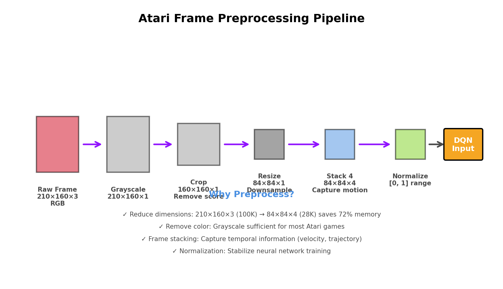
Preprocessing for Atari Games
To make learning feasible, Atari frames are preprocessed:
Frame Preprocessing Pipeline
python
def preprocess_frame(frame):
    # 1. Convert to grayscale
    gray = cv2.cvtColor(frame, cv2.COLOR_RGB2GRAY)

    # 2. Resize to 84×84
    resized = cv2.resize(gray, (84, 84))

    # 3. Normalize pixel values to [0, 1]
    normalized = resized / 255.0

    return normalized
Frame Stacking
Stack 4 consecutive frames to capture motion:
yaml
Frame 1: Position at t-3
Frame 2: Position at t-2
Frame 3: Position at t-1
Frame 4: Position at t
         ↓
State: 84×84×4 tensor (captures velocity implicitly)
Why stack frames?
- Single frame = no velocity information (ball could be moving left or right)
- 4 frames = agent sees direction and speed of movement
DQN Extensions and Improvements
Double DQN
Problem: Standard DQN overestimates Q-values due to max operator.
Standard DQN target:
css
y = r + γ * max_a' Q(s', a'; θ⁻)
Double DQN target:
css
a* = argmax_a' Q(s', a'; θ)      # Select action with online network
y = r + γ * Q(s', a*; θ⁻)         # Evaluate with target network
Benefit: Reduces overestimation bias, more stable learning.
Dueling DQN
Architecture: Split Q-network into value and advantage streams.
scss
Q(s,a) = V(s) + [A(s,a) - mean_a' A(s,a')]
Where:
- V(s): Value of being in state s
- A(s,a): Advantage of taking action a in state s
Benefit: Learns state values independently of actions, better for states where action choice doesn't matter.
Prioritized Experience Replay
Idea: Sample important transitions more frequently.
Priority: TD error magnitude |δ| = |r + γ max Q(s',a') - Q(s,a)|
Benefit: Learn faster from surprising transitions.
Common Failure Modes
One. Catastrophic Forgetting
Symptom: Agent learns well, then suddenly forgets and performance drops.
Causes:
- Replay buffer too small (old experiences discarded)
- Learning rate too high
- Target network updated too frequently
Fixes:
- Increase replay buffer size (100k -> 1M)
- Reduce learning rate
- Increase target update frequency
2. Overestimation Bias
Symptom: Q-values grow unrealistically large, unstable learning.
Cause: Max operator in Q-learning inherently overestimates.
Fixes:
- Use Double DQN
- Clip rewards to [-1, 1]
- Add gradient clipping
3. No Learning Signal
Symptom: Q-values stay near zero, no improvement.
Causes:
- Sparse rewards (agent rarely reaches goal)
- Poor exploration (epsilon too low)
- Insufficient training (buffer not filled)
Fixes:
- Reward shaping (add intermediate rewards)
- Increase epsilon or exploration duration
- Fill replay buffer before training
4. Instability / Divergence
Symptom: Q-values explode, agent performance collapses.
Causes:
- Learning rate too high
- No target network
- Correlated samples (no replay buffer)
Fixes:
- Reduce learning rate (0.001 -> 0.0001)
- Implement target network
- Use experience replay
- Add gradient clipping
DQN on Atari Games: Breakthrough Results
DQN Paper (2015)
Performance:
- 29/49 Atari games: Human-level or better
- Breakout: 400+ average score (human expert: ~30)
- Space Invaders: 1,000+ average score (human: ~1,200)
- Pong: Near-perfect play (+20 average reward)
Training:
- 50 million frames (~38 hours of gameplay)
- 3-4 days on GPU
Games Where DQN Excelled
- Breakout: Learned to tunnel through bricks (emergent strategy!)
- Pong: Mastered perfect returns
- Enduro: Consistent high scores
Games Where DQN Struggled
- Ms. Pac-Man: Requires long-term planning (>100 steps)
- Montezuma's Revenge: Extremely sparse rewards
- Pitfall: Exploration challenge (huge state space)
Advantages of DQN
- Scales to high-dimensional spaces: Images, complex observations
- End-to-end learning: Raw pixels -> actions (no feature engineering)
- Data efficient: Experience replay reuses data
- Stable: Target networks prevent oscillations
- Proven: Achieved human-level performance on many Atari games
Limitations of DQN
- Sample inefficiency: Still requires millions of frames
- Discrete actions only: Can't handle continuous action spaces directly
- Overestimation: Q-values tend to be optimistic
- Sparse rewards: Struggles with exploration in large environments
- Memory requirements: Large replay buffers (GBs of memory)
Key Takeaways
- Function approximation extends Q-Learning to large/continuous state spaces
- Experience replay breaks correlation, enables data reuse
- Target networks stabilize learning by fixing targets temporarily
- DQN architecture: Convolutional layers for images, fully connected for vectors
- Hyperparameters matter: Learning rate, buffer size, target update frequency
- Extensions improve: Double DQN, Dueling DQN, Prioritized Replay
- Preprocessing critical: Grayscale, resize, frame stacking for Atari
Looking Ahead
DQN launched the deep RL revolution, but it has limitations:
- Lesson 4: Policy gradient methods for continuous actions
- Lesson 5: Actor-critic methods combining value and policy
- Lesson 6: PPO for stable, sample-efficient learning
Next lesson, we'll explore a fundamentally different approach: directly learning policies instead of value functions.
Summary
- Deep Q-Networks use neural networks to approximate Q-values for large state spaces
- Experience replay stores transitions in a buffer and samples randomly for training
- Target networks stabilize learning by freezing Q-value targets for several steps
- DQN architecture: Convolutional layers for images, fully connected for low-dimensional states
- Hyperparameters significantly affect training stability and performance
- Extensions (Double DQN, Dueling DQN) improve upon vanilla DQN
- Applications: Atari games, robotics simulation, game playing