Regression

:dart: Learning Objectives

By the end of this lesson, you will be able to:

• Understand what regression is and when to use it
• Identify independent and dependent variables
• Implement simple and multiple linear regression
• Create visualizations of regression models
• Evaluate regression model performance

:information_source: Regression is a supervised machine learning algorithm that predicts numerical values. Think of it as a smart calculator that learns patterns from data to make predictions about numbers!

Regression helps us predict numerical outputs based on data we've seen before. For example, it can predict tomorrow's temperature based on today's weather patterns.

Since regression is a supervised learning algorithm, we need labeled datasets (data with known answers) to train our model.

:star2: Applications of Regression

Regression helps solve real-world problems:

• Health & Fitness: Predict a person's weight based on their height and exercise habits
• Business: Forecast product prices based on manufacturing costs and market demand
• Real Estate: Estimate house prices using location, size, and number of rooms

:memo: In this chapter, we'll learn about Linear Regression - one of the most popular and easy-to-understand regression algorithms!

Linear Regression

:information_source: Linear Regression is a statistical model that finds the best straight line through your data points. It helps predict how one thing changes when another thing changes!

:mag: Independent and Dependent Variables

Before diving into Linear Regression, let's understand two important concepts:

Independent Variables (x)

Independent variables are the inputs you control or change. Think of them as the "cause" in a cause-and-effect relationship.

Examples:

• Plant experiment: Amount of water you give to a plant
• Health study: Number of hours someone exercises tip Remember: Independent variables are what YOU change or control. We use "x" to represent them in math!

Dependent Variables (y)

Dependent variables are the results that change based on your inputs. They "depend" on the independent variables.

Examples:

• Plant experiment: How tall the plant grows (depends on water amount)
• Health study: Person's fitness level (depends on exercise hours)

:bulb: Remember: Dependent variables are what you MEASURE or observe. We use "y" to represent them in math!

:bar_chart: Types of Linear Regression

Linear Regression comes in three flavors:

1. Simple Linear Regression: Uses ONE independent variable to make predictions
2. Multiple Linear Regression: Uses MULTIPLE independent variables for better predictions
3. Polynomial Linear Regression: Uses curved lines instead of straight lines (we'll learn this later!)

:dart: Simple Linear Regression

Simple Linear Regression uses just ONE independent variable to predict ONE dependent variable. It's like finding the best straight line through your data points!

The Magic Formula

The simple linear regression formula is:

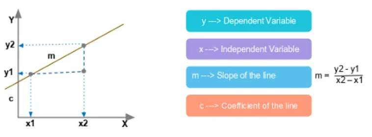
text

y = mx + c

Let's break this down:

• x: Your independent variable (what you know)
• y: Your dependent variable (what you want to predict)
• m: The slope - tells you how steep your line is
• c: The y-intercept - where your line crosses the y-axis

Understanding Slopes

The slope (m) determines how your line looks:

note Quick Guide to Slopes:

• Positive slope (m > 0): As x goes up, y goes up too! :chart_with_upwards_trend:
• Negative slope (m < 0): As x goes up, y goes down :chart_with_downwards_trend:
• Zero slope (m = 0): y stays the same no matter what x does ->
• Undefined slope: The line goes straight up and down ↕️

How Linear Regression Works

The algorithm learns from your data by following these steps:

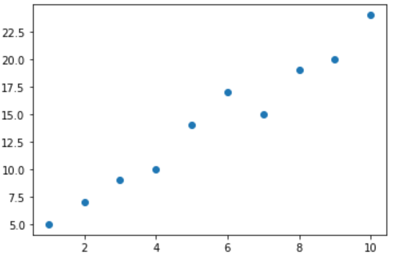
1. Step One: Plot the data :emoji: The algorithm places all your data points on a graph

   

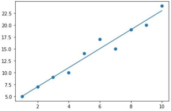
2. Step 2: Find the best line :emoji: It finds the line that fits your data points best (closest to all points)

   

3. Step 3: Make predictions :dart: Use the line to predict new values!

   

Real-World Applications

Simple Linear Regression helps solve problems like:

• Agriculture: Predict crop yield based on water amount :emoji:
• Health: Estimate a person's weight from their height :bar_chart:
• Sales: Forecast revenue based on advertising spending :emoji:

:rocket: Multiple Linear Regression

Multiple Linear Regression is like Simple Linear Regression's big sibling! Instead of using just one factor, it uses MANY factors to make better predictions.

The Enhanced Formula

y = m1x1 + m2x2 + m3x3 + ... + c

Here's what each part means:

• x1, x2, x3: Different independent variables (multiple factors)
• y: What we're trying to predict
• m1, m2, m3: How much each factor affects the result
• c: The starting point (y-intercept)

:bulb: Think of it like baking a cake! :emoji:

• Simple Linear Regression: Only considers flour amount
• Multiple Linear Regression: Considers flour, sugar, eggs, AND baking time!

Visualization Challenge

Unlike simple linear regression, we can't easily draw multiple linear regression on a 2D graph because we're working with many dimensions!

Real-World Applications

Multiple Linear Regression solves complex problems:

• Smart Farming: Predict crop yield using water amount, fertilizer, AND temperature :emoji:
• Science Experiments: Calculate liquid density from mass AND volume :emoji:
• Weather Forecasting: Predict temperature using humidity, wind speed, AND pressure :emoji:️

:computer: Implementation of Linear Regression

Let's build our own Linear Regression model! Follow these simple steps:

Step One: Import and Create Model

from sklearn.linear_model import LinearRegression
model = LinearRegression()

Step 2: Train the Model

Feed your training data to the model so it can learn:

model.fit(x_train, y_train)

Step 3: Check the Slope (m)

See how steep your line is:

print(model.coef_)

[2.30952381]

Step 4: Check the Y-intercept (c)

Find where your line crosses the y-axis:

print(model.intercept_)

-0.8928571428571441

Step 5: Test Your Model

Check how well your model performs (closer to 1.0 is better!):

model.score(x_test, y_test)

0.8016846856454839

:memo: A score of 0.80 means your model is 80% accurate - that's pretty good! :tada:

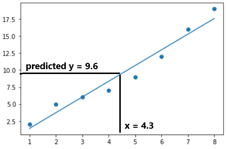
Step 6: Make Predictions

Use your trained model to predict new values:

python

list(model.predict([[1],[2],[3]]))

text

[1.4166666666666656, 3.7261904761904754, 6.035714285714285]

:chart_with_upwards_trend: Plotting the Linear Regression Graph

Let's visualize our model! We'll use Matplotlib to create beautiful graphs. tip This only works for Simple Linear Regression (one x variable). Multiple Linear Regression needs more complex visualization!

Step One: Import Matplotlib

import matplotlib.pyplot as plt

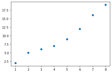
Step 2: Plot Your Data Points

Create a scatter plot to see your data:

plt.scatter(x, y)

Step 3: Get Your Line Parameters

Retrieve the slope and y-intercept from your trained model:

m = model.coef_
c = model.intercept_

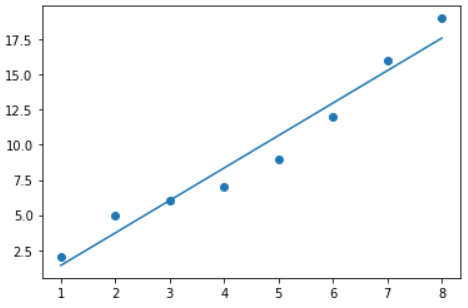
Step 4: Draw the Line of Best Fit

Add your regression line to the graph:

plt.plot(x_train, m*x_train+c)
plt.show()

Step 5: Make It Pretty! :sparkles:

Add labels and titles to make your graph more informative:

plt.title('Graph of X against Y')    # Add a title
plt.xlabel('X-values')                # Label x-axis
plt.ylabel('Y-values')                # Label y-axis

:memo: Note Want to learn more about styling graphs? Check out the Data Visualization chapter!

:emoji: Summary

Let's recap what we learned about regression:

:information_source: Key Takeaways:

1. Regression predicts numerical values from data patterns
2. Simple Linear Regression uses one factor to predict outcomes
3. Multiple Linear Regression uses many factors for better predictions
4. The line of best fit represents the relationship between variables
5. We can evaluate models using the score method (0-1, higher is better)

:emoji: Video

:emoji: AI Prompt

Code with AI: Try using AI to build a regression model.

Prompts to try:

• "Write Python code to implement a linear regression model using scikit-learn."
• "How can I evaluate the performance of a regression model?"
• "Show me how to visualize a regression line with matplotlib."
• "Explain the difference between simple and multiple linear regression with examples."

:dart: Practice Activities

1. Predict Your Grade: Create a simple linear regression model to predict test scores based on study hours
2. Weather Predictor: Use multiple linear regression to predict temperature based on humidity and wind speed
3. Graph Challenge: Create a beautiful visualization of your regression model with proper labels and colors
4. Real Data: Find a real dataset online and apply regression to solve a problem you're interested in!